Robust Graph SLAM using ICP-Based LIDAR Scan Matching and EKF-IMU preintegration

Collaborator(s): Atharva Patwe

This work aims to implement a robust Simultaneous Localization and Mapping algorithm on a turtlebot platform using onboard sensors - 2D Lidar, Wheel Encoders, and Magnetometer compass. This study explores the implementation of online SLAM and full SLAM using factor graphs, specifically leveraging the Georgia Tech Smoothing and Mapping (GTSAM) library on a turtlebot robot platform with the Robot Operating System (ROS). Our study also incorporates the Closed form ICP covariance estimation method proposed by an existing work.

Methodology

The factors of the graph are estimated with the help of two separate navigators

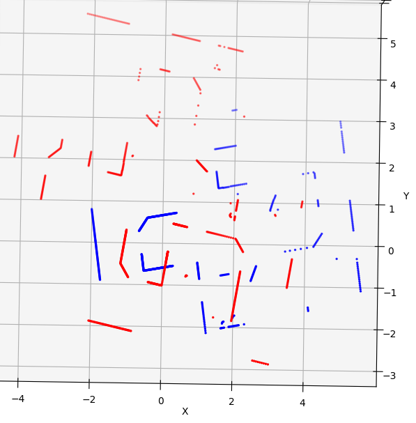
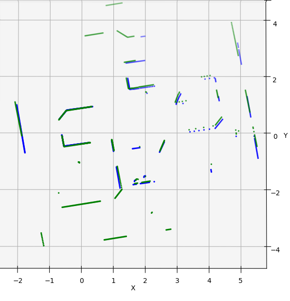
Scan Matching Navigator: the scans obtained from the lidar are converted into the robot base frame after and registered with all the scan saved earlier using transformations obtained from matching. The pointcloud matching is carried out by ICP algorithm giving the transformation between the scans which are then added to the graph as Pose 2D constraints with some uncertainty.
EKF Odometry: the odometry factors are estimated using an Extended Kalman Filter (EKF). The EKF predicts the robot’s pose based on encoder readings and updates this prediction with compass measurements.

The sampling frequency of the wheel encoder and compass is relatively high, in the range of 100-200 Hz, allowing the EKF Odometry Navigator to update odometry at a high rate. The Lidar, however, operates at a much lower frequency. To obtain meaningful scan matching results, the robot needs to have some displacement between subsequent Lidar scans. Therefore, new poses are added at the frequency of Lidar matches. Between two Lidar matches, the odometry data is preintegrated and added once along with the scan matching factor.

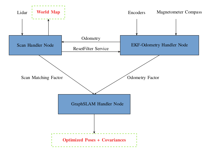
Graph SLAM ROS Package Architecture.

The uncertainty of the odometry is calculated by the EKF by tuning the uncertainties of the encoders and compass. The final covariance matrix of the odometry is used to estimate the Gaussian noise model for that factor. On the other hand, since ICP does not have a built-in covariance estimation procedure, the uncertainty of the scan matching factor is estimated using a method derived from the work of A. Censi. After adding all the factors with their uncertainties and variables, the graph is optimized. For Online applications, sparse nonlinear incremental optimization (iSAM2) is used which achieves improvements in efficiency through incremental variable re-ordering and fluid relinearization, eliminating the need for periodic batch steps as proposed by Kaess. For the full SLAM problem, more accurate solvers, such as the Levenberg-Marquardt solver, are used. One drawback of using iSAM2 in GTSAM is that, as an incremental solver, it cannot estimate the uncertainties of the robot’s past poses. The optimized poses are then used to register all the scans again to build the world map.

Results

ICP Alignment

Point Cloud Comparisons before and after ICP: (Left) Source Pointcloud in red at timestamp k and Target Pointcloud in blue and timestamp k-1, (Right) Aligned Pointcloud in green of timestamp k and Target Pointcloud in blue at time k-1.

Graph SLAM Simulation Results

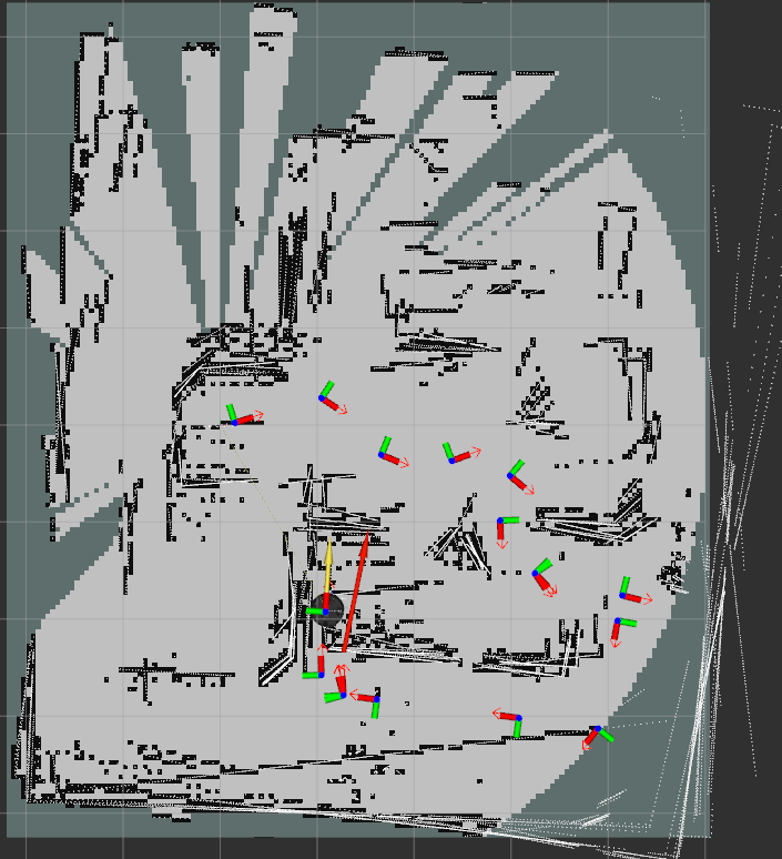
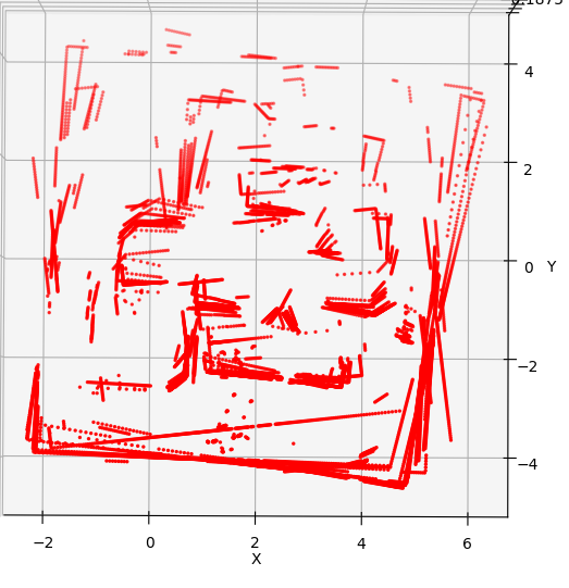
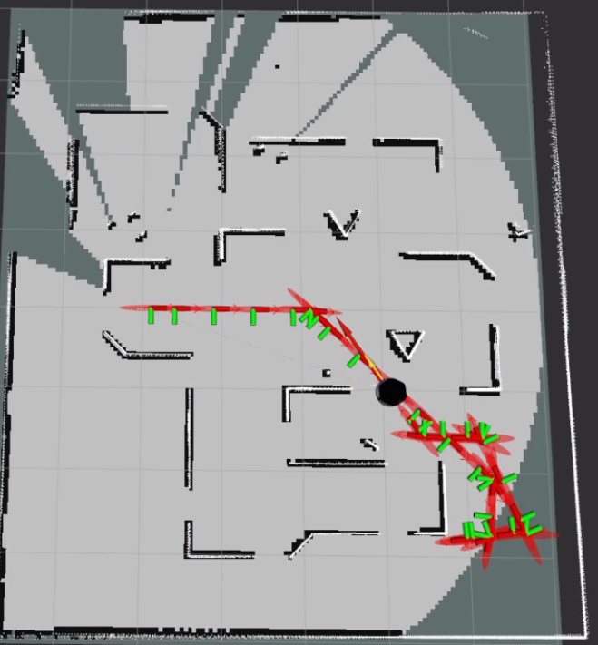
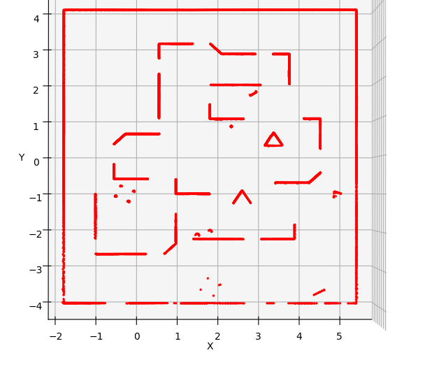
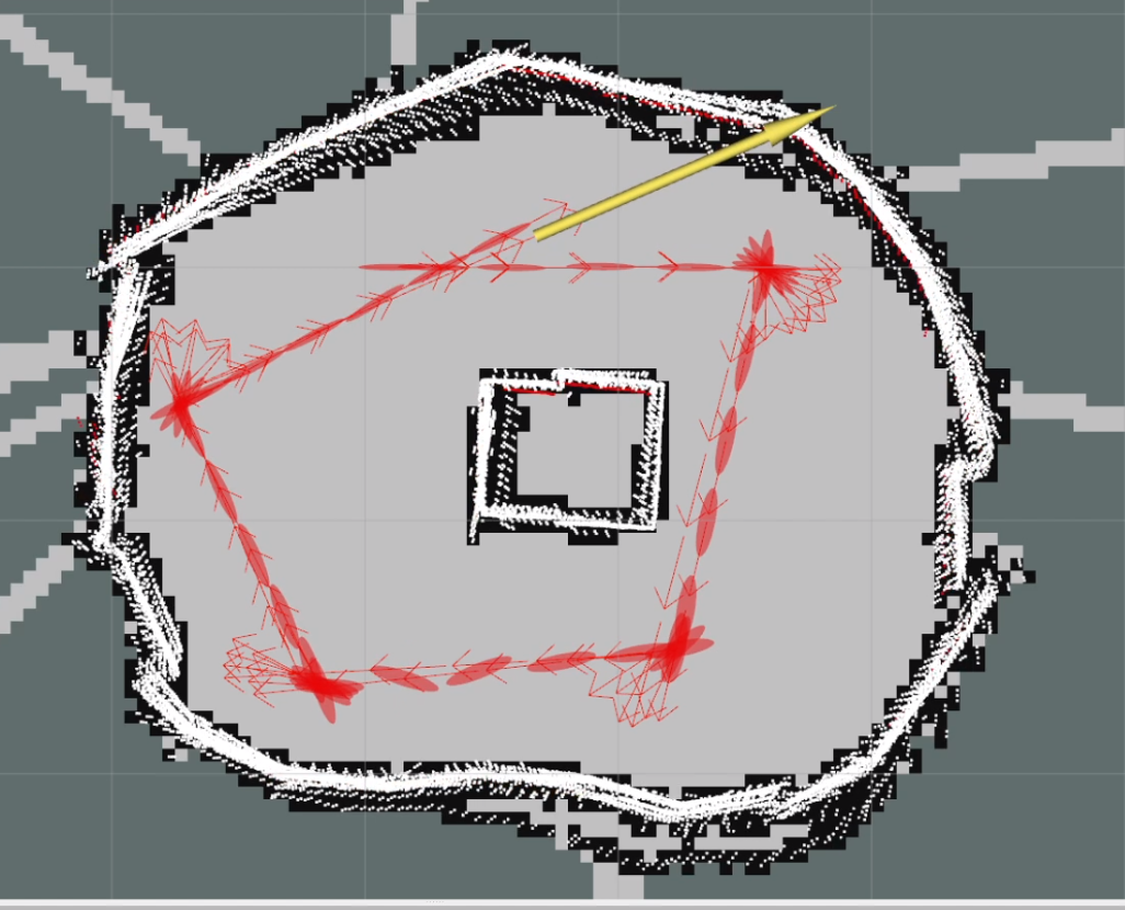
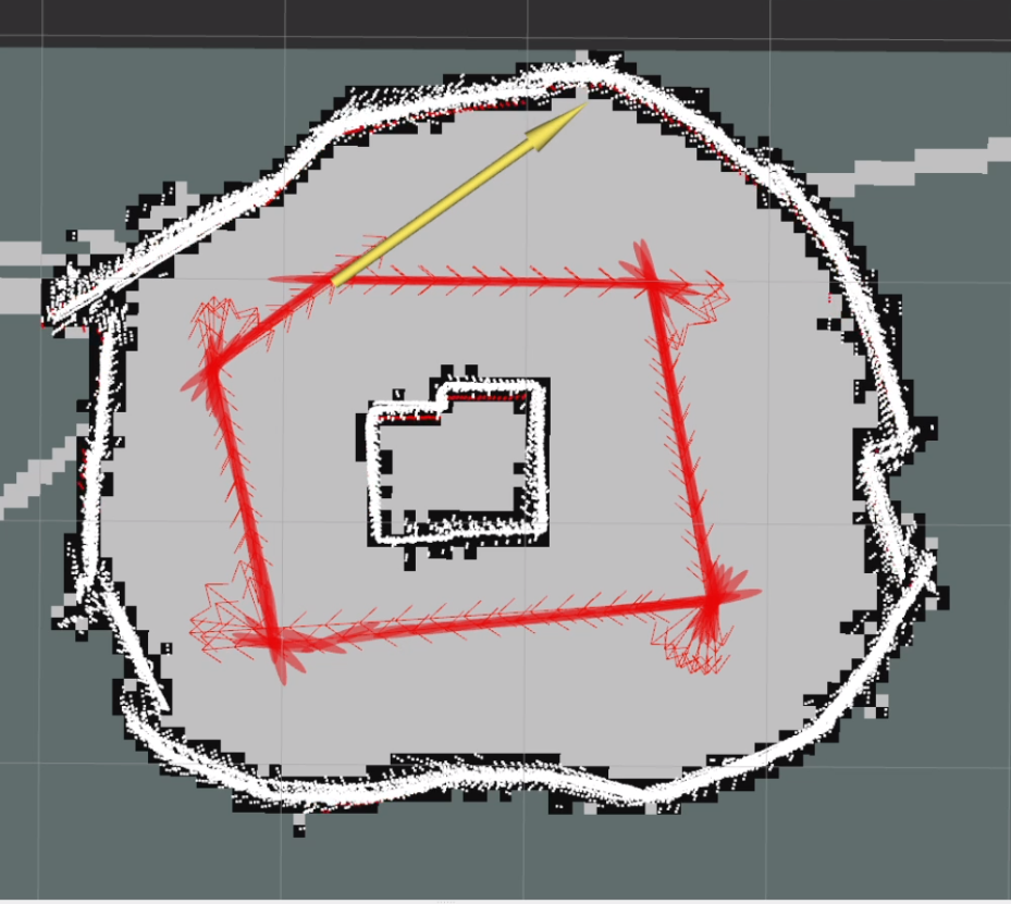
Simulation: World Point Cloud Constructed Using Dead Reckoning Only(Odometry). Red and Green Axes Indicate Factor Graph Keyframes, Red Arrow Represents Robot Pose Calculated by Graph SLAM, and Yellow Arrow Indicates Ground Truth

Simulation: World Point Cloud Constructed Using Pose Graph Optimization via Graph SLAM. Red and Green Axes Indicate Factor Graph Keyframes, Red Arrow Represents Robot Pose Calculated by Graph SLAM, and Yellow Arrow Indicates Ground Truth

Graph SLAM Experimental Validation and Results Loop Closure: For experimental validation of the loop closure condition and its effects, a map depicted in Figure below was created. In SLAM, loop closure refers to the process of identifying and closing loops in the robot’s trajectory as it explores an environment. When a robot revisits a previously visited location, loop closure algorithms detect this revisitation point and reconcile the new data with the existing map, effectively ’closing’ the loop. When the robot revisits a keyframe, the uncertainties associated with the keyframes in the graph naturally decrease as the drift is corrected. To demonstrate this effect, the robot was traversed along a circular track in the map. This behavior is evident in Figures below, where as the robot progresses through the map, the uncertainty ellipsoid (depicted in red) gradually expands until it approaches the starting pose. Upon reaching close to the previous keyframe, a new factor is introduced between the current keyframe and the previous keyframes. During the optimization process, this factor facilitates the correction of drift, resulting in a more confident pose graph. This correction is visually indicated by the reduction in the size of the ellipsoids, signifying improved certainty in the robot’s localization and mapping.

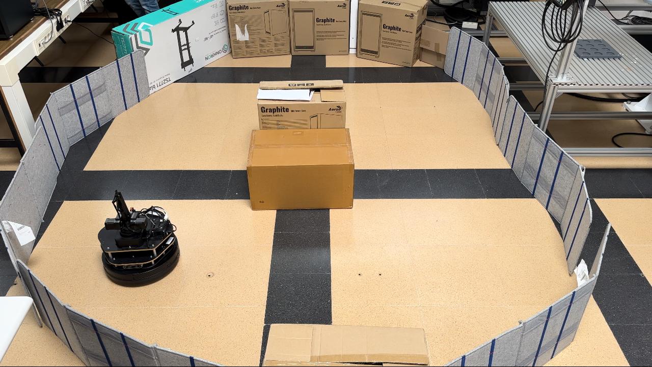
(Left) Loop-Closure test environment. (Middle) Turtlebot2 Graph SLAM Results without Closed form ICP Covariance Estimation Method. (Right) Turtlebot2 Graph SLAM Results with ICP Covariance Estimation Method.

Evaluation Graph SLAM for mapping in an environment with obstacles: